Technical knowledge base Study Notes Scala 401.03 - Partitioning and shuffling

401.03 - Partitioning and shuffling

Shuffling

What happens when you call a groupBy or a groupByKey operation, when the data is distributed?

Example:

val pairs = sc.parallelize(List((1, "one), (2, "two"), (3, "three")))
pairs.groupByKey()
// res2: org.apache.spark.rdd.RDD[(Int, Iterable[String])]
//   = ShuffledRDD[16] at groupByKey at <console>:37

In order to perform this operation, data has to be moved over the network in order to be aggregated. This data move is called shuffling.

Shuffles can incur enormous performance hits, because Spark has to move data around the network, which is slow.

Another example. Given:

case class CFFPurchase(customerId: Int, destination: String, price: Double)

Assume we have an RDD of the purchases that customers made in the past month:

val purchasesRdd: RDD[CFFPurchase] = sc.textFile(...)

We want to calculate how many trips and how much money was spent by each individual customer over the course of the month.

val purchasesPerMonth = purchasesRdd.map(p =>(p.customerId, p.price))   // Pair RDD
                .groupByKey()    // RDD[K, Iterable[V]]
                ,map(p => (p._1, (p._2,size, p._2.sum)))
                .collect()

What happens with the data in the following scenario:

val purchases = List(
    CFFPurchase(100, "Geneva", 22.25),
    CFFPurchase(300, "Zurich", 42.50),
    CFFPurchase(100, "Fribourg", 12.40),
    CFFPurchase(200, "St. Gallen", 8.20),
    CFFPurchase(100, "Lucerne", 31.60),
    CFFPurchase(300, "Basel", 16.20))

How would the data be distributed on 3 computation nodes:

CFFPurchase(100, "Geneva", 22.25), CFFPurchase(100, "Lucerne", 31.60)
CFFPurchase(100, "Fribourg", 12.40), CFFPurchase(200, "St. Gallen", 8.20)
CFFPurchase(300, "Zurich", 42.5), CFFPurchase(300, "Basel", 16.20)

map:

(100, 22.25), (100, 31.60)
(100, 12.40), (200, 8.20)
(300, 42.50), (300, (16.20)

groupByKey (requires shuffling):

(100, [22.25, 31.60, 12.40])
(200, [8.20])
(300, [42.50, 16.20])

We don't want to be sending all the data over the network if it's not absolutely required. Too much network communication kills the performance.

In order to minimize the amount of data that gets sent over the network during shuffling, we could use a reduceByKey operation before grouping. reduceByKey can be thought as a combination of first doing a groupByKey and then reducing all the values grouped by key.

def reduceByKey(func: (V, V) => V: RDD[(K, V)]

Here is how the code would look like, using reduceByKey:

val purchasesPerMonth = purchasesRdd.map(p => (p.customerId, (1, p.price)))
    .reduceByKey((v1, v2) => (v1._1 + v2._1, v1._2 + v2._2))
    .collect()

How does this look on the cluster?

How would the data be distributed on 3 computation nodes:

CFFPurchase(100, "Geneva", 22.25), CFFPurchase(100, "Lucerne", 31.60)
CFFPurchase(100, "Fribourg", 12.40), CFFPurchase(200, "St. Gallen", 8.20)
CFFPurchase(300, "Zurich", 42.5), CFFPurchase(300, "Basel", 16.20)

map:

(100, 22.25), (100, 31.60)
(100, 12.40), (200, 8.20)
(300, 42.50), (300, (16.20)

reduceByKey (requires some shuffling). This executes in two stages: first on the mapper side:

(100, (2, 53,85))
(100, (1, 12.40)), (200, (1, 8.20))
(300, (2, 58.70))

then between the nodes:

(100, (3, 67,25))
(200, (1, 8.20))
(300, (2, 58.70))

The amount of data that gets moved over the network is minimized.

Partitioning

We saw that operations like *groupByKey require shuffling. Grouping all values of key-value pairs with the same key requires collecting all key-value pairs with the same key on the same node. But how does Spark know which key to put on which node?

Data within an RDD is split into several partitions. Partitions have the following properties:

Partitions never span multiple nodes. Tuples in the same partition are guaranteed to be on the same machine;
Each nde contains one ore more partitions;
The number of partitions to use is configurable. By default, it equals the total number of cores on all executor nodes;

Two kinds of partitioning are available in Spark:

Hash partitioning
Range partitioning

Customizing a partitioning is only possible on Pair RDDs !

Hash partitioning

Back to our example. Given a Pair RDD that should be grouped:

val purchasesPerMonth = purchasesRdd.map(p =>(p.customerId, p.price))   // Pair RDD
                .groupByKey()    // RDD[K, Iterable[V]]

groupByKey will first compute per tuple (k, v) its partition p:

p = k.hashCode() % numPartitions

Then, all tuples in the same partition p are sent to the machine hosting p.

Hash partitioning attempts to spread the data evenly across partitions based on the key.

Range partitioning

Pair RDDs may contain keys that have an ordering defined (ex: Int, Char, String). For such RDDs, range partitioning may be more efficient. Using a range partitioner, keys are partitioned accordng to:

an ordering for keys
a set of sorted ranges of keys

Tuples with keys in the same range appear on the same machine.

Example: consider that we want to use a hash partitioning for it an RDD with the following keys:

[8, 96, 240, 400, 401, 800]

and a desired number of partitions of 4. Let's assume that the hash function is the identity:

(n.hashCode() == n)

We end up with the following partitions:

- [8, 96, 240, 400, 800]
- [401]
- 
-

The result is a very unbalanced distribution that hurts peformance.

Using range partitioning can improve the distribution significantly. The set of ranges for our RDD will be:

- [1, 200]
- [201, 400]
- [401, 600]
- [601, 800]

and the data will be partitioned as follows:

- [8, 96]
- [240, 400]
- [401]
- [800]

The resulting partitioning is more balanced.

Customizing the partitioner

a) by calling partitionBy on an RDD, providing a specific Partitioner; b) using transformations that return RDDs with specific partitioners;

Invoking partitionBy creates an RDD with a specified partitioner. Example:

val pairs = purchasesRdd.map(p => (p.customerId, p.price))

val tunedPartitioner = new RangePartitioner(8, pairs)  // 8 is the number of partitions
val partitioned = pairs.partitionBy(tunedPartitioner).persist()

The call to persist() prevents Spark partitioning the data over and over again.

Creating a RangePartitioner requires:

1) Specifying the desired number of partitions; 2) Providing a Pair RDD with ordered keys. This RDD is sampled by Spark to create a suitable set of sorted ranges; 3) The result of partitionBy should be persisted in order to prevent repeated partitioning of the data;

Partitioning data using transformations

Partitioner from parent RDD

Pair RDDs that are the result of a transformation on a partitioned Pair RDD typically is configured to use the hash partitioner that was used to construct it.

Automatically-set partitioners

Some operations on RDDs automatically result in an RDD with a known partitioner (when it makes sense). For example, by default, when using sortByKey, a RangePartitioner is used. Also, the default partitioner when using groupByKey is a HashPartitioner.

Operations that hold to and propagate a partitioner:

cogroup
groupWith
join
leftOuterJoin
rightOuterJoin
groupByKey
reduceByKey
foldByKey
combineByKey
partitionBy
sort
mapValues (if parent has a partitioner)
flatMapValues (if parent has a partitioner)
filter (if parent has a partitioner)

All other operations (this includes map and flatMap) will produce a result without a partitioner. This is because these operations can completely change the type of the key. This isn't the case in, say, mapValues where the key is preserved.

Optimizing with Partitioners

Partitioning can bring enormous performance gains, especially in the face of shuffles. For instance, using range partitioners in our previous example, when using reduceByKey, we can end up with no shuffling at all!!!

val pairs = purchasesRdd.map(p => (p.customerId, p.price))
val tunedPartitioner = new rangePartitioner(8, pairs)

val partitioned = pairs.partitionBy(tunedPartitioner).persist()

val purchasesPerCustomer = partitioned.map(p => (p._1, (1, p._2)))

val purchasesPerMonth = purchasesPerCustomer
    .reduceByKey((v1, v2) => (v1._1 + v2._1, v1._2 + v2._2))
    .collect()

Because all tuples for the same customer will be located on each node, the computation time will be in the order of 10x faster.

Let's look at another example. Consider an application that keeps a large table of user information in memory:

userData - BIG, containing (UserID, UserInfo) pairs, where UserInfo contains a list of topics that the user is subscribed to

The application periodically combines this BIG table with a smaller file representing events that happened in the past 5 minutes:

events - small, containing (UserID, LinkInfo) pairs for users who have clicked a link on a website in the past 5 minutes;

For example, we might wish to count how many users visited a link that was not one of their subscribed topics. We can perform this combination using a join operation, which can be used to group the UserInfo and LinkInfo pairs for each UserID by key.

val sc = new SparkContext(...)
val userData = sc.sequenceFile[UserID, UserInfo]("hdfs://...")
    .persist()

def processNewLogs(logFileName: String) {
    val events = sc.sequenceFile[UserID, LinkInfo](logFileName)
    val joined = userData.join(events)  //RDD[UserID, (UserInfo, LinkInfo))]
    val offTopicVisists = joined.filter {
        case (userId, (userInfo, linkInfo)) =>  // expand the tuple
            !userInfo.topics.contains(linkInfo.topic)
    }.count()
    println("Number of visits to non-subscribed topics: " + offTopicVisits;
}

This implementation is very inefficient. The join operation doesn't know anything about how the keys are partitioned in the datasets. The operation will hash all of the keys in both datasets, sending elements with the same hash value across the network to the same machine and then join together the elements with the samke key on that machine. This happens even though the user data in the BIG file doesn't change.

Fixing this is easy, just by using partitionBy on the BIG userData RDD at the start of the program.

val userData = sc.sequenceFile[UserID, UserInfo]("hdfs://...")
    .partitionBy(new HashPartitioner(100))
    .persist()

Since we called partitionBy, Spark now knows that userData is hash-partitioned and calls to join will take advantage of this information. When calling the join operation, Spark will shuffle only the events RDD, sending events with each particular UserID to the machine that contains the corresponding hash partition of the userData.

Recall the example using groupByKey:

val purchasesPerMonth = purchasesRdd.map(p =>(p.customerId, p.price))   // Pair RDD
                .groupByKey()    // RDD[K, Iterable[V]]

Grouping all values of key-value pairs with the same key requires collecting all key-value pairs with the same key on the same machine. But grouping is done using a hash partitioner with default parameters. The result RDD, purchasesPerCust will use the same partitioner that was use to construct it.

Rule of thumb: a shuffle can occur when the resulting RDD depends on other elements from the same RDD or another RDD. You can also figure out whether a shuffle has been planned and executed via:

1) the return type of certain transformations, like ShuffledRDD[366] 2) using function toDebugString to see its execution plan:

partitioned.reduceByKey((v1, v2) => (v1._1 + v2._1, v1._2 + v2._2))
    .toDebugString

// res9: String = 
// (8) MapPartitionRDD[622] at reduceByKey
//     | ShuffledRDD[615] at partitionBy
//     |    CacedPartitions: 8; MemorySize: 1754.8 MB; DiskSize: 0.0 B

Operations that might cause shuffles

cogroup
groupWith
join
leftOuterJoin
rightOuterJoin
groupByKey
reduceByKey
combineByKey
distinct
intersection
repartition
coalesce

There are a few ways to use operations that might cause a shuffle and to still avoid much or all of the network shuffling:

reduceByKey on a pre-partitioned RDD will cause the values to be computed locally , requiring only the final reduced value to be sent from the worker to the driver;
join called on two RDDs that are pre-partitioned with the same partitioner and cached on the same machine will cause the join to be computed locally, with no shuffling across the network;

Wide vs Narrow dependencies

Some transformations are significantly more expensive in terms of latency than others (for instance: requiring lots of data to be transferred over the network unnecessarily.

Lineage

Computations on RDDs are represented as a lineage graph; a Directed Acyclic Graph (DAG) representing the computations done on the RDD.

Example:

val rdd = sc.textFile(...)
val filtered = rdd.map(...).filter(...).persist()
val count = filtered.count()
val reduced = filtered.reduce(...)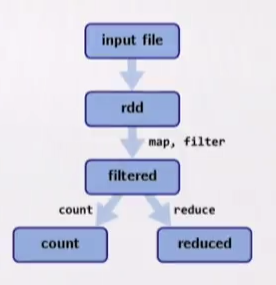

Spark will analyze the DAG in order to optimize.

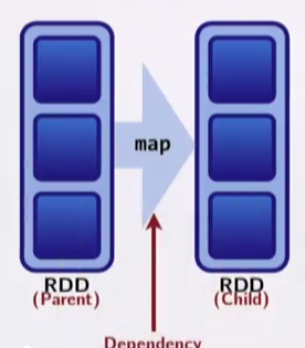
RDDs are represented as:

Partitions - atomic pieces of the dataset. One or many per compute node;
Dependencies - models relationships between this RDDs and its partitions with the RDD(s) it was derived from;
A function (lambda) for computing the dataset based on its parent RDD;
Metadata about its partitioning scheme and data placement;

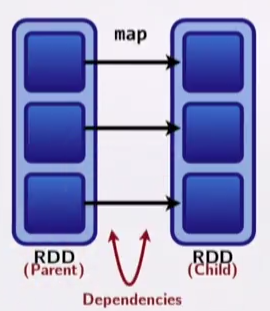
Previously we arrived at the following rule of thumb: a shuffle can occur when the resulting RDD depends on other elements from the same RDD or another RDD.

In fact dependencies encode when data must move across the network.

Transformations cause shuffles. Transformations can have two kind of dependencies:

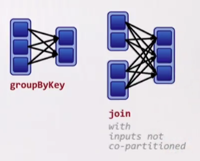
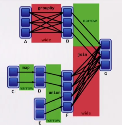
Narrow dependencies - each partition of the parent RDD is used by at most one partition of the child RDD. Fast! No shuffle necessary. Optimizations like pipelining are possible;

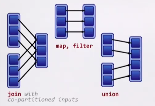
Wide dependencies - each partition of the parent RDD may be depended on by multiple child partitions. Slow! Requires all or some data to be shuffled over the network;

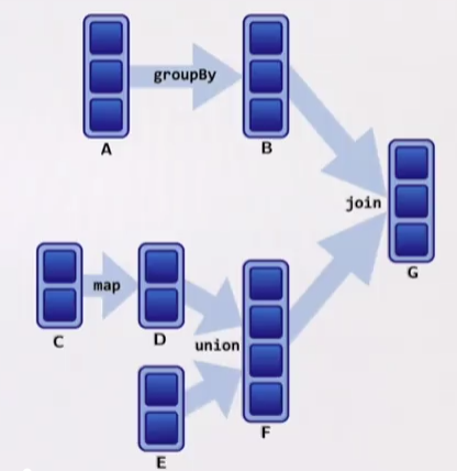
Example: let's assume we have the following DAG:

Transformations with narrow dependencies:

map
mapValues
flatMap
filter
mapPartitions
mapPartitionsWithIndex

Transformations with wide dependencies( might cause a shuffle):

cogroup
groupWith
join
leftOuterJoin
rightOuterJoin
groupByKey
reduceByKey
combineByKey
distinct
intersection
repartition
coalesce

We can find out more about the dependencies of an RDD by invoking the dependencies() method:

Narrow dependency objects: OneToOneDependency, PruneDependency, RangeDependency
Wide dependency objects: ShuffleDependency

Example:

val wordsRdd = sc.parallelize(largeList)
val pairs = wordsRdd.map(c => (c, 1))
    .groupByKey()
    .dependencies

// pairs: Seq[org.apache.spark.Dependency[_]] =
// List(org.apache.spark.ShuffleDependency@12345)

The toDebugString() method prints out a visualization of the RDD's lineage, and other information related to scheduling.Indentations in the output separate groups of narrow transformations that may be pipelined together and wide transformations that require shuffles. These groupings are called stages.

val wordsRdd = sc.parallelize(largeList)
val pairs = wordsRdd.map(c => (c, 1))
    .groupByKey()
    .toDebugString

// pairs: String
// (8) ShuffledRDD[219]  at groupByKey
// +- (8) MapPartitionsRDD[218] at map
//      | ParallelCollection[217] at parallelize

Fault tolerance

Lineage graphs are the key to fault tolerance in Spark. Functional programming enables the fault tolerance:

RDDs are immutable;
We use high-order functions such as map, flatMap, filter to do functional transformations on this immutable data;
A function for computing the dataset based on its parent RDDs also is a part of the RDD representation;

This allows recomputing at any given time any subset of transformations in the entire lineage graph. In this way Spark can recover from failure by recomputing lost partitions from the lineage graph.